## KL Divergence Function for multivariate Gaussian
def kl_divergence(mu1, mu2, sigma1, sigma2):
    diff_mu = mu2 - mu1
    sigma2_inv = inv(sigma2)

    term1 = diff_mu.T @ sigma2_inv @ diff_mu
    term2 = np.trace(sigma2_inv @ sigma1)
    term3 = -np.log(np.linalg.det(sigma1) / np.linalg.det(sigma2))
    term4 = -len(mu1)

return 0.5 * (term1 + term2 + term3 + term4)While studying Machine Learning, I often come across the concept of KL Divergence. It is omnipresent, at least in the field of ML, and I often find myself studying the concept over and over again, so I think that it’d be useful to (finally and) formally note down for the sake of self-reference and revision. Hopefully others will find it useful too. Of course this is by no means everything about KL Divergence. Feedback are more than welcome.
Definition
Given two distributions \(P\) and \(Q\) of a continuous random variable \(x\), the KL Divergence between \(P\) and \(Q\) is defined as:
KL Divergence Definition
\[\begin{equation} \label{kl-def} \int_\mathcal{X} P(x) \log \dfrac{P(x)}{Q(x)}dx. \end{equation}\]
An example: KL Divergence between two Gaussian distributions
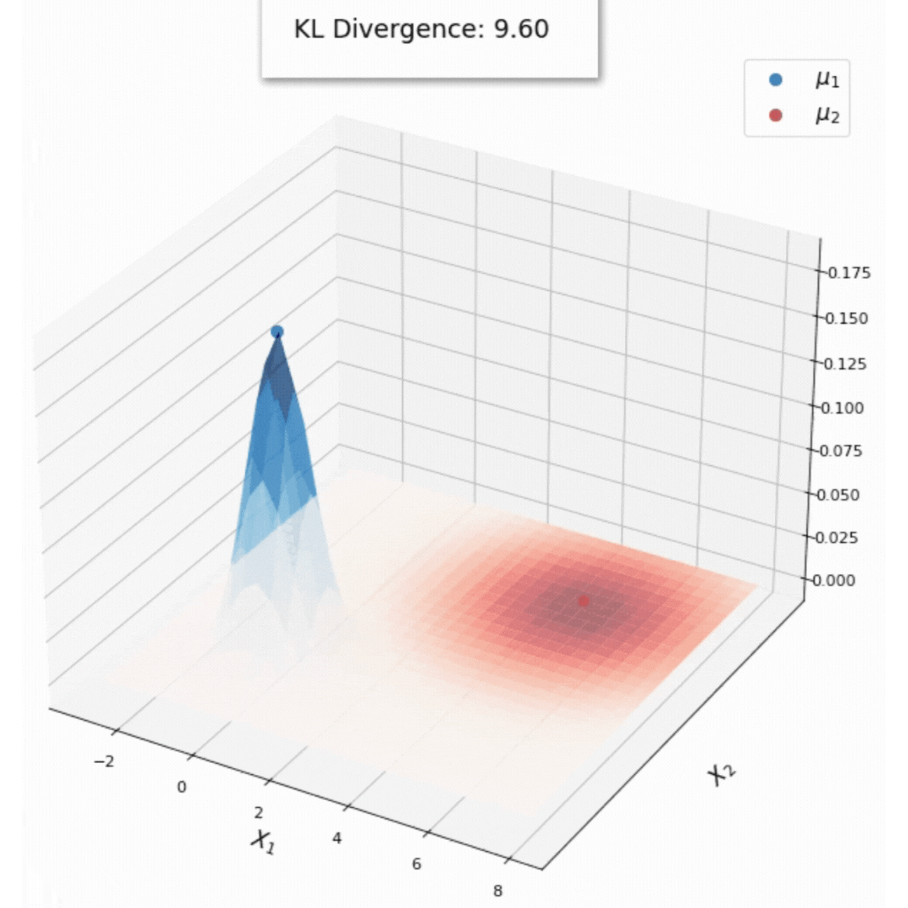
Suppose we are given two Gaussian distributions \(P \sim \mathcal{N}(\mu_1, \Sigma_1)\); \(Q \sim \mathcal{N}(\mu_2, \Sigma_2)\), and a random vector \(x \in \mathbb{R}^{n \times 1}\), the KL Divergence between \(P\) and \(Q\) has the following analytic form:
\[ D_{\text{KL}}(P(x) \| Q(x)) = \dfrac{1}{2} \left[(\mu_2 - \mu_1)^T \Sigma_2^{-1} (\mu_2 - \mu_1) + \text{tr}(\Sigma_2^{-1}\Sigma_1^1) - \log \dfrac{|\Sigma_1|}{|\Sigma_2|} - n \right] \]
Additionally, consider the following derivation:
\[\begin{aligned} D_{\text{KL}}(P \| Q) &= \int_\mathcal{X} P(x) \log \dfrac{P(x)}{Q(x)} dx && \text{(from } \eqref{kl-def}) \\ &= \int_\mathcal{X} \mathcal{N}(x; \mu_1, \Sigma_1) \log \dfrac{\mathcal{N}(x; \mu_1, \Sigma_1)}{\mathcal{N}(x; \mu_2, \Sigma_2)} \\ &= \underset{x \sim P(x)}{\mathbb{E}}\left[\log \dfrac{\mathcal{N}(x; \mu_1, \Sigma_1)}{\mathcal{N}(x; \mu_2, \Sigma_2)} \right]. \end{aligned}\]Plugging in the multivariate Gaussian PDF, we have:
\[\begin{aligned} \underset{x \sim P(x)}{\mathbb{E}}\left[\log \dfrac{\mathcal{N}(x; \mu_1, \Sigma_1)}{\mathcal{N}(x; \mu_2, \Sigma_2)} \right] &= \underset{x \sim P(x)}{\mathbb{E}}\left[\dfrac{\frac{1}{\sqrt{2(\pi)^n|\Sigma_1|}} \exp(-\frac{1}{2} (x-\mu_1)^T \Sigma_1^{-1} (x-\mu_1))}{\frac{1}{\sqrt{(2\pi)^n|\Sigma_2|}} \exp(-\frac{1}{2} (x-\mu_2)^T \Sigma_2^{-1} (x-\mu_2))} \right] \\ &= \dfrac{1}{2}\underset{x \sim P(x)}{\mathbb{E}}\left[ \log \dfrac{|\Sigma_2|}{|\Sigma_1|} - (x-\mu_1)^T \Sigma_1^{-1} (x-\mu_1) + (x-\mu_2)^T \Sigma_2^{-1} (x-\mu_2) \right] \end{aligned}\]Using the fact that \(x = \text{tr}(x)\) and \(\text{tr}(ABC) = \text{tr}(BCA)\), we have:
\[\begin{aligned} \underset{x \sim P(x)}{\mathbb{E}}\left[\log \dfrac{\mathcal{N}(x; \mu_1, \Sigma_1)}{\mathcal{N}(x; \mu_2, \Sigma_2)} \right] &= \dfrac{1}{2}\underset{x \sim P(x)}{\mathbb{E}}\left[ \log \dfrac{|\Sigma_2|}{|\Sigma_1|} - \text{tr}[(x-\mu_1)^T \Sigma_1^{-1} (x-\mu_1)] + \text{tr}[(x-\mu_2)^T \Sigma_2^{-1} (x-\mu_2)] \right] \\ &= \dfrac{1}{2}\underset{x \sim P(x)}{\mathbb{E}}\left[ \log \dfrac{|\Sigma_2|}{|\Sigma_1|} - \text{tr}[\Sigma_1^{-1}(x-\mu_1)(x-\mu_1)^T] + \text{tr}[\Sigma_2^{-1}(xx^T - 2\mu_2 x^T + \mu_2 \mu_2^T)] \right] \\ &= \dfrac{1}{2}\left[ \log \dfrac{|\Sigma_2|}{|\Sigma_1|} - \text{tr}[\Sigma_1^{-1}\underset{x \sim P(x)}{\mathbb{E}}[(x-\mu_1)(x-\mu_1)^T]] + \text{tr}[\Sigma_2^{-1}\underset{x \sim P(x)}{\mathbb{E}}[(xx^T - 2\mu_2 x^T + \mu_2 \mu_2^T)]] \right] \\ &= \dfrac{1}{2}\left[ \log \dfrac{|\Sigma_2|}{|\Sigma_1|} - \text{tr}[\Sigma_1^{-1} \Sigma_1] + \text{tr}[\Sigma_2^{-1}[\underset{x \sim P(x)}{\mathbb{E}}[(xx^T)] - 2\underset{x \sim P(x)}{\mathbb{E}}[\mu_2 x^T] + \underset{x \sim P(x)}{\mathbb{E}}[(\mu_2 \mu_2^T)]] \right] \\ &= \dfrac{1}{2}\left[ \log \dfrac{|\Sigma_2|}{|\Sigma_1|} - n + \text{tr}[\Sigma_2^{-1}[\Sigma_1 + \mu_1\mu_1^T - 2\underset{x \sim P(x)}{\mathbb{E}}[\mu_2 \mu_1^T] + \underset{x \sim P(x)}{\mathbb{E}}[(\mu_2 \mu_2^T)]] \right] \\ &= \dfrac{1}{2}\left[ \log \dfrac{|\Sigma_2|}{|\Sigma_1|} - n + \text{tr}[\Sigma_2^{-1}\Sigma_1] + \text{tr}[\mu_1^T \Sigma_2^{-1} \mu_1 - 2[\mu_1^T \Sigma_2^{-1} \mu_2] +(\mu_2^T \Sigma_2^{-1} \mu_2)]] \right] \\ &= \dfrac{1}{2}\left[ \log \dfrac{|\Sigma_2|}{|\Sigma_1|} - n + \text{tr}[\Sigma_2^{-1}\Sigma_1] + (\mu_2 - \mu_1)^T \Sigma_2^{-1} (\mu_2 - \mu_1) \right] \\ &= \dfrac{1}{2} \left[(\mu_2 - \mu_1)^T \Sigma_2^{-1} (\mu_2 - \mu_1) + \text{tr}(\Sigma_2^{-1}\Sigma_1^1) - \log \dfrac{|\Sigma_1|}{|\Sigma_2|} - n \right] \end{aligned}\]In code, this could be implemented as:
KL Divergence of distributions in the exponential family
The exponential family is a particular family of probability distributions that can be rewritten in the following form:
\[ p(x \vert \eta) = h(x)\exp(\eta^T \mathcal{T}(x) - \mathcal{A}(\eta)). \]
where \(h(x)\) is the base measure, \(\eta\) is the natural parameters, \(\mathcal{T}(x)\) is the sufficient statistic, and \(\mathcal{A}(\eta)\) is the log-partition function.
The KL divergence between two distributions from the same exponential family can be expressed in a closed-form analytic expression. Consider the following derivation:
\[\begin{aligned} D_{\text{KL}}(p(x \vert \eta_1) \| p(x \vert \eta_2)) &= \int p(x \vert \eta_1) \log \dfrac{p(x \vert \eta_1)}{p(x \vert \eta_2)}dx \\ &= \int p(x \vert \eta_1) - \mathcal{A}(\eta_1)) \log \dfrac{h(x)\exp(\eta_1^T \mathcal{T}(x) - \mathcal{A}(\eta_1))}{h(x)\exp(\eta_2^T \mathcal{T}(x) - \mathcal{A}(\eta_2))} dx \\ &= \int p(x \vert \eta_1) [\eta_1^T \mathcal{T}(x) - \mathcal{A}(\eta_1) - \eta_2^T \mathcal{T}(x) + \mathcal{A}(\eta_2)] dx\\ &= \int p(x \vert \eta_1) [\mathcal{T}(x) (\eta_1^T-\eta_2^T ) -\mathcal{A}(\eta_1)+\mathcal{A}(\eta_2)] dx\\ &= \underset{p(x \vert \eta_1)}{\mathbb{E}}[(\eta_1^T-\eta_2^T )] -\mathcal{A}(\eta_1)+\mathcal{A}(\eta_2) \end{aligned}\]Therefore, the KL divergence between two distributions from the same exponential family, parameterized by their natural parameters \(\eta_1\) and \(\eta_2\) is \(\underset{p(x \vert \eta_1)}{\mathbb{E}}[(\eta_1^T-\eta_2^T )] -\mathcal{A}(\eta_1)+\mathcal{A}(\eta_2)\).
As a quick sanity check, we can calculate the KL divergence between two Poisson distributions, both in the naive way and under the lens of the closed form for KL divergence of distributions in the exponential family.
We first start by showing that the Poisson distribution with parameter \(\lambda\) is in the exponential family by rewriting its PMF as:
\[\begin{aligned} P(x; \lambda) &= \sum_{x} \dfrac{\lambda^x \exp(-\lambda)}{x!} \\ &= \frac{1}{x!} \exp(x \log \lambda - \lambda) \\ \end{aligned}\]Therefore, the Poisson distribution is in the exponential family, where \(\eta = \log \lambda\), \(\mathcal{T}(x) = x\), \(\mathcal{A}(\eta) = \lambda = \exp(x)\), and \(h(x)=\frac{1}{x!}\).
We now calculate the KL Divergence between two Poisson distributions parameterized by \(\lambda_1\) and \(\lambda_2\):
\[\begin{aligned} D_{\text{KL}}(p(x; \lambda_1) \| p(x; \lambda_2)) &= \sum_x p(x; \lambda_1) \log \dfrac{p(x; \lambda_1)}{p(x; \lambda_2)} && \text{(by definition)} \\ &= \sum_x \dfrac{\lambda_1^x \exp(-\lambda_1)}{x!} \log \dfrac{\lambda_1^x \exp(-\lambda_1)}{\lambda_2^x \exp(-\lambda_2)} && \text{(by plugging in the Poisson PMF)} \\ &= \sum_x \dfrac{\lambda_1^x \exp(-\lambda_1)}{x!} \left(x \log \dfrac{\lambda_1}{\lambda_2} + \lambda_2 - \lambda_1 \right) \\ &= \sum_x \dfrac{\lambda_1^x \exp(-\lambda_1)}{x!} \left(x \log \dfrac{\lambda_1}{\lambda_2}\right) + (\lambda_2 - \lambda_1)\sum_x \dfrac{\lambda_1^x \exp(-\lambda_1)}{x!} && \text{(by rearranging the sum)} \\ &= \underset{p(x; \eta_1)}{\mathbb{E}}[x] \log \dfrac{\lambda_1}{\lambda_2} + (\lambda_2 - \lambda_1) && \\ &= \lambda_1 \log \dfrac{\lambda_1}{\lambda_2} + (\lambda_2 - \lambda_1) \label{eq1} \end{aligned}\]Therefore we have:
\[ \begin{equation} \label{eq:poisson} D_{\text{KL}}(p(x; \lambda_1) \| p(x; \lambda_2)) = \lambda_1 \log \dfrac{\lambda_1}{\lambda_2} + (\lambda_2 - \lambda_1) \end{equation} \]
Now, consider the closed-form expression for the KL Divergence between two distributions from the same exponential family:
\[ D_{\text{KL}}(p(x \vert \eta_1) \| p(x \vert \eta_2)) = \underset{p(x \vert \eta_1)}{\mathbb{E}}[x](\eta_1-\eta_2)^T -\mathcal{A}(\eta_1)+\mathcal{A}(\eta_2) \]
Plugging in each component for two Poisson distributions, we have:
\[\begin{aligned} D_{\text{KL}}(p(x; \lambda_1) \| p(x; \lambda_2)) &= (\log \lambda_1 - \log \lambda_2) \underset{p(x; \lambda_1)}{\mathbb{E}}(x) - \lambda_1 + \lambda_2 \\ &= \lambda_1 \log \dfrac{\lambda_1}{\lambda_2} + \lambda_2 - \lambda_1, \end{aligned}\]which is analogous to the previous closed-form expression.
KL Divergence Minimization meets MLE
Recall that in Maximum Likelihood Estimation, our goal is to find the parameters \(\theta^*\) that maximizes the likelihood function, i.e.:
\[\begin{aligned} \theta^*_{\text{MLE}} &= \underset{\theta}{\text{argmin }} p_\theta(x^{(1)}, x^{(2)}, \cdots, x^{(n)}) \\ &= \underset{\theta}{\text{argmax }} \prod_{i=1}^{n} p_\theta(x^{(i)}) \quad \text{(suppose that $x^{(i)}$ are i.i.d.)}\\ &= \underset{\theta}{\text{argmax }} \log \prod_{i=1}^{n} p_\theta(x^{(i)}) \\ &= \underset{\theta}{\text{argmax }} \sum_{i=1}^{n} \log p_\theta(x^{(i)}). \end{aligned}\]We now show that minimizing the KL divergence between two distributions is equivalent to MLE. Suppose our data is drawn from some arbitrary distribution \(P_{\text{data}}\), our goal is to find the parameters \(\theta\) such that \(P_\theta\) is as close to \(P_\text{data}\) as possible. This can be achieved by minimizing the KL Divergence between \(P_{\text{data}}\) and \(P_\theta\). The objective can thus be written as:
\[\begin{aligned} \theta^* &= \underset{\theta}{\text{argmin }} D_\text{KL}(P_\text{data} (x) \| P_\theta (x)) \\ &= \underset{\theta}{\text{argmin }} \int_{x \in \mathcal{X}} P_\text{data}(x) \log \dfrac{P_\text{data}(x)}{P_\theta (x)}dx \\ &= \underset{\theta}{\text{argmin }} \underset{x \sim P_\text{data}(x)}{\mathbb{E}} \left[\log \dfrac{P_\text{data}(x)}{P_\theta (x)}\right] \\ &= \underset{\theta}{\text{argmin }} \underset{x \sim P_\text{data}(x)}{\mathbb{E}} [\log P_\text{data}(x) - \log P_\theta (x)] \\ &= \underset{\theta}{\text{argmin }} \underset{x \sim P_\text{data}(x)}{\mathbb{E}} [\log P_\text{data}(x)] - \underset{x \sim P_\text{data}(x)}{\mathbb{E}}[\log P_\theta (x)] \\ &= \underset{\theta}{\text{argmin }} \underset{x \sim P_\text{data}(x)}{-\mathbb{E}}[\log P_\theta (x)] \\ &= \underset{\theta}{\text{argmax }} \underset{x \sim P_\text{data}(x)}{\mathbb{E}}[\log P_\theta (x)] \\ &\approx \underset{\theta}{\text{argmax }} \dfrac{1}{n}\sum_{i=1}^{n} \log p_\theta(x^{(i)}). \end{aligned}\]Now, we observe that the \(\frac{1}{n}\) term does not affect the optimization since it is a constant scalar factor independent of \(\theta\). Maximizing \(\frac{1}{n} \sum_{i=1}^n \log p_\theta(x^{(i)})\) is equivalent to maximizing \(\sum_{i=1}^n \log p_\theta(x^{(i)})\). Therefore:
\[\theta^*_{\text{MLE}} = \arg\max_{\theta} \sum_{i=1}^n \log p_\theta(x^{(i)})\]
is equivalent to minimizing the KL divergence:
\[\theta^* = \arg\min_{\theta} D_{KL}(P_\text{data} \| P_\theta).\]
KL Divergence Properties
Non-negativity
Using Jensen’s inequality, we can show that the KL Divergence is non-negative. Consider the following derivation:
\[\begin{aligned} D_{\text{KL}}(P \| Q) &= \sum_{x} \log P(x) \dfrac{P(x)}{Q(x)} \\ &= -\sum_{x} \log P(x) \dfrac{Q(x)}{P(x)} \\ &= \underset{x \sim P(x)}{\mathbb{E}}\left[-\log \dfrac{Q(x)}{P(x)}\right] \\ &\geq -\log \underset{x \sim P(x)}{\mathbb{E}}\left[\dfrac{Q(x)}{P(x)}\right] \\ &= -\log \sum_x P(x) \dfrac{Q(x)}{P(x)} \\ &= -\log \sum_x Q(x) \\ &= -\log 1 = 0. \end{aligned}\]Therefore \(D_{\text{KL}}(P(x) \| Q(x)) \geq 0\) for all \(x\).
Asymmetry
In the intuition section, we see why the KL divergence needs to be asymmetric. We now formally prove that it is indeed asymmetric. We can simply do so by taking one concrete example and calculate the KL divergence between the two distributions, if these two values are not equal, then it suffices that the KL divergence is not symmetric.
Let \(P(x)\) and \(Q(x)\) be two distributions defined as:
\[ P(x) = \begin{cases} -1, & \text{w.p. } 0.5 \\ 1, & \text{w.p. } 0.5 \end{cases} \quad \text{ and } Q(x) = \begin{cases} -1, & \text{w.p. } 0.1 \\ 1, & \text{w.p. } 0.9 \end{cases} \]
You can easily verify that \(D_{\text{KL}}(P \| Q) = 0.5 \cdot \ln\left(\frac{0.5}{0.1}\right) + 0.5 \cdot \ln\left(\frac{0.5}{0.9}\right)\) and \(D_{\text{KL}}(Q \| P) = 0.1 \cdot \ln\left(\frac{0.1}{0.5}\right) + 0.9 \cdot \ln\left(\frac{0.9}{0.5}\right),\) and they are not equal.
Convexity
A continuous function \(f\) is said to be convex if
\[ \begin{equation} \label{eq:convex1} f(\lambda x + (1-\lambda)y) \leq \lambda f(x) + (1-\lambda) f(y) \text{ for } 0 \leq \lambda \leq 1. \end{equation} \]
This equation can be generalized when we have two input variables. In particular, for a convex function \(f(x,y)\) and two inputs \((x_1, y_1)\); \((x_2, y_2)\), it holds that:
\[ f(\lambda x_1 + (1-\lambda)x_2, \lambda y_1 + (1-\lambda)y_2) \leq \lambda f(x_1, y_1) + (1-\lambda) f(x_2, y_2) \text{ for } 0 \leq \lambda \leq 1 \]
Thus, to prove that the KL divergence is convex, this means that we have to prove the following statement:
\[ \begin{equation} \label{eq-kl-convex} D_{\text{KL}}[\lambda p_1 + (1-\lambda)p_2 \| \lambda q_1 + (1-\lambda)q_2] \leq \lambda D_{\text{KL}}[p_1 \| q_1] + (1-\lambda) D_{\text{KL}}(p_2 \| q_2). \end{equation} \]
To do this, we first need to know the Log sum inequality, which states that:
\[ \left(\sum_{i=1}^n a_i \right)\log \dfrac{\sum_{i=1}^n a_i}{\sum_{i=1}^n b_i} \leq \sum_{i=1}^n \left( a_i \log \dfrac{a_i}{b_i}\right). \]
For example, if we have \(a = a_1 + a_2\) and \(b= b_1+b_2\), what the Log sum inequality is telling us is the following:
\[ \begin{equation} \label{eq:log-sum} ({a_1} + {a_2}) \log \dfrac{a_1+a_2}{b_1 + b_2} \leq {a_1} \log \dfrac{a_1}{b_1} + {a_2} \log \dfrac{a_2}{b_2}. \end{equation} \]
Let \({p_{\lambda} = \lambda p_1 + (1-\lambda) p_2}\) and \({q_{\lambda} = \lambda q_1 + (1-\lambda) q_2}\). Applying the Log sum inequality, it holds that:
\[\begin{aligned} D_{\text{KL}} (p_{\lambda} \| q_{\lambda}) &= \sum_{x \in \mathcal{X}} p_{\lambda}(x) \log \frac{p_{\lambda}(x)}{q_{\lambda}(x)} && \text{(by definition)} \\ &\geq \sum_{x \in \mathcal{X}} p_{\lambda}(x) \log \frac{\sum_{x \in \mathcal{X}} p_{\lambda}(x)}{\sum_{x \in \mathcal{X}} q_{\lambda}(x)} && \text{(by log-sum inequality)}. \end{aligned}\]Expanding out \({p_{\lambda}}\)$ and $\({q_{\lambda}}\), we have:
\[\begin{aligned} D_{\text{KL}} \big(\lambda p_1 + (1-\lambda) p_2 \, \big\| \, \lambda q_1 + (1-\lambda) q_2 \big) &= \sum_{x \in \mathcal{X}} \big(\lambda p_1(x) + (1-\lambda) p_2(x)\big) \log \frac{\lambda p_1(x) + (1-\lambda) p_2(x)}{\lambda q_1(x) + (1-\lambda) q_2(x)} \\ &\leq \sum_{x \in \mathcal{X}} \left(\lambda p_1(x) \log \frac{\lambda p_1(x)}{\lambda q_1(x)} + (1-\lambda) p_2(x) \log \frac{(1-\lambda) p_2(x)}{(1-\lambda) q_2(x)}\right) \\ &= \lambda \sum_{x \in \mathcal{X}} p_1(x) \log \frac{p_1(x)}{q_1(x)} + (1-\lambda) \sum_{x \in \mathcal{X}} p_2(x) \log \frac{p_2(x)}{q_2(x)} \\ &= \lambda D_{\text{KL}}(p_1 \| q_1) + (1-\lambda) D_{\text{KL}}(p_2 \| q_2). \end{aligned}\]Here, we’re applying the Log-sum inequality, where \(a_1 = {\lambda p_1}\), \(a_2 = {(1-\lambda) p_2}\), \(b_1 = {\lambda q_1}\), and \(b_2 = {(1-\lambda) q_2}\).
KL Divergence Chain rule
We now show the KL Divergence chain rule, i.e. it holds that:
\[D_{\text{KL}}(P(X,Y) \| Q(X, Y)) = D_{\text{KL}}(P(X) \| Q(X)) + D_{\text{KL}}(P(Y \vert X) \| Q(Y \vert X)).\]
\[\begin{aligned} D_{\text{KL}}(P(X,Y) \| Q(X, Y)) &= \sum_X \sum_Y P(x,y) \log \frac{P(x, y)}{Q(x, y)} \\ &= \sum_X \sum_Y P(x) P(y \vert x) \log \frac{P(x)P(y \vert x)}{Q(x) Q(y \vert x)} \\ &= \sum_X \sum_Y P(x) P(y \vert x) \left(\log \frac{P(x)}{Q(x) } + \log \frac{P(y \vert x)}{Q(y \vert x)}\right) \\ &= \sum_X P(x) \log \frac{P(x)}{Q(x) } \sum_Y P(y \vert x) + \sum_Y P(y \vert x) \log \frac{P(y \vert x)}{Q(y \vert x)} \sum_X P(x) \\ &= D_{\text{KL}}(P(X) \| Q(X)) + D_{\text{KL}}(P(Y \vert X) \| Q(Y \vert X)) \end{aligned}\]This result also generalizes for \(n\) random variables, i.e.:
\[D_{\text{KL}}(P(X_1, \cdots, X_n) \| Q(X_1, \cdots, X_n)) = \sum_{i=1}^n D_{\text{KL}}(P(X_i \vert X_1, \cdots, X_{i-1}) \| Q(X_i \vert X_1, \cdots, X_{i-1})).\]
Approximating the KL Divergence with Fisher Information
The main derivation for this section is from Section 5.1.9 in Probabilistic Machine Learning: Advanced Topics by Kelvin P. Murphy.
The Fisher Information Matrix (FIM) is defined to be a covariance of the score function \(\nabla_\theta \log p(x \vert \theta)\), i.e.:
\[ F(\theta) = \underset{x \sim p_\theta (x)}{\mathbb{E}} [\nabla_\theta \log p(x \vert \theta) \nabla_\theta \log p(x \vert \theta)^T]. \]
Suppose we want to compute the KL Divergence term between two distributions \(p_\theta(x)\) and \(p_\theta'(x)\), where \(\theta' = \theta + \delta\). Then we have:
\[\begin{aligned} D_{\text{KL}}(p_\theta (x) \| p_{\theta'}(x)) = \underset{p_\theta(x)}{\mathbb{E}}[\log p_\theta(x) - \log p_{\theta'}(x)] \end{aligned}\]Now consider the second order Taylor expansion, we have:
\[\begin{aligned} D_{\text{KL}}(p_\theta (x) \| p_{\theta'}(x)) &\approx -\delta^T \underset{p_\theta(x)}{\mathbb{E}}[\nabla \log p_\theta(x)] - \dfrac{1}{2} \delta^T \underset{p_\theta(x)}{\mathbb{E}}[\nabla^2 \log p_\theta(x)] \delta \\ &= - \dfrac{1}{2} \delta^T \underset{p_\theta(x)}{\mathbb{E}}[\nabla \log p_\theta(x) \nabla \log p_\theta(x)^T] \delta \\ &= -\dfrac{1}{2} \delta^T \mathbf{F} \delta \end{aligned}\]The second-order Taylor expansion of KL divergence shows that, locally, it takes a quadratic form involving the Fisher Information Matrix \(\mathbf{F}\), which underscores its role in shaping the geometry of the parameter space, linking KL divergence to natural gradient methods and statistical inference.