Change log
- Feb 10: Add Elephant in the room.
- Feb 09: Move back from al-folio to Quarto :).
For a long time, traditional ML models focus only on one modality, such as text, image, or audio. As humans, we are capable of dealing with multiple modalities at the same time. The human experience is multimodal. We see, hear, smell, and touch. In addition, the Internet and many applications nowadays are multimodal. For example, we can rarely see any webpages that contain only text or images, and we hardly watch any video without any sound. The explosion of Internet data comes with vast data resources and availability that we can use to train advanced AI models.
While there are many different modalities that have been considered in the ML community, in this blog post, we will focus on vision and text modality. There are many different ways that we can use to categorize Vision-Language Models, either based on their training paradigms, input/output modalities, or pre-training objectives. Following Bordes et al. (2024) [1], one way of categorizing different VLMs is via their training paradigms, which include 1) contrastive; 2) masking; 3) generative; and 4) using pre-trained backbones. These methods are, however, not mutually exclusive, there have been work that combine two or more training paradigms. Among the most popular VLMs, VILA [2] and its variants are a family of models that focus on efficiency while maintaining impressive performance.
VILA
Given the explosion of LLMs in recent years, it is natural to come up with ways to extend such LLMs to be able to work with the visual modality (eg images and videos). VILA [2] is a VLM introduced by NVIDIA and MIT that is based on such approach by integrating visual and textual information. It is pre-trained based on the recipes that the authors observe. At its core, VILA consists of three main components, including 1) a visual encoder, 2) an LLM, and 3) a projector. The vision backbone is CLIP visual encoder [3] and the LLM used is Llama2-7b and Llama2-13b [4]. A projector acts as a mapping to connect the images and text embeddings onto the same space, it can either be as simple as a linear layer or MLP, or as complicated as a Transformer block. VILA takes visual and text inputs and generates text outputs. This section outlines several design choices to improve the model’s performance based on empirical observation.
Full fine-tuning or visual prompt tuning ?
The two common methods that have often been used to augment LLMs with visual inputs is either to 1) fine-tune the LLM with the visual tokens (also referred to as (full) fine-tuning) or 2) only train the visual input while freezing the weights of the LLM (often known as (visual) prompt tuning). The prompt-tuning approach treats the visual input projector as a way to “prompt” the LLM with visual embeddings while keeping the text-only model intact. It can be thought of as a “translator” between the vision encoder and the text-only LLM, effectively acting as the “prompt.”
The question of whether to use the former or latter approach comes with different tradeoffs. While fine-tuning is essential for the VLM to inherit the LLMs’ in-context learning ability, it comes with the risk of catastrophic forgetting, where the model’s ability degrades on text-only tasks. Such a problem can be prevented by using prompt tuning, however, this leads to poor performance and degrades in-context learning capabilities.
| Setting | PreT | SFT | Projector | OKVQA (0s) | OKVQA (4s) | TextVQA (0s) | TextVQA (4s) | COCO (0s) | COCO (4s) | Flickr (0s) | Flickr (4s) | Average (0s) | Average (4s) |
|---|---|---|---|---|---|---|---|---|---|---|---|---|---|
| a) | ✗ | ✗ | Transformer | 10.4 | 19.2 | 14.8 | 23.1 | 17.4 | 60.2 | 11.0 | 47.4 | 13.4 | 37.5 |
| b) | ✗ | ✓ | Transformer | 47.1 | 47.7 | 37.2 | 36.6 | 109.4 | 88.0 | 73.6 | 58.1 | 66.8 | 57.6 |
| c) | ✓ | ✓ | Transformer | 44.8 | 49.8 | 38.5 | 38.8 | 112.3 | 113.5 | 71.5 | 72.9 | 66.8 | 68.8 |
| d) | ✓ | ✓ | Linear | 45.2 | 50.3 | 39.7 | 40.2 | 115.7 | 118.5 | 74.2 | 74.7 | 68.7 | 70.9 |
Full fine-tuning is important. In the VILA paper, the authors did experiments with different settings (A-D, where setting a) and b) focus on prompt tuning (LLM is frozen); c) and d) involve fine-tuning (LLM is updated). Table 1 shows that freezing the LLM during pre-training does not negatively impact zero-shot accuracy, but it results in a reduced ability for in-context learning. Another observation from this experiment is that using a simple projector (linear layer) leads to better performance. The hypothesis is that using a simple projector enforces the LLM to learn more from visual tokens, and thus the model can generalize better.
The benefits of full finetuning approach is, however, depends on the size of the downstream dataset size, as shown by Cheng et al. (2024) in Figure 1.
Training Data
Training data is one of the most important aspects of training VLMs 1. Some common practices to preprocess the image-text data are to 1) remove the duplicate, 2) balance the labels, 3) prune (removing the data pairs where the captions do not match with the image), and 4) improve the captions with other LLMs.
The two most common types of data used for training VLMs include interleaved image-text data and image-text pair data (i.e. the images and their corresponding captions). In the VILA paper, the authors train the model with different types of data to analyze their influence on the model’s performance.
Interleaved or Image-text pair Data ?
The VILA paper shows that interleaved image-text data like MMC4 [6] is more effective regarding training VLM because it prevents the model from catastrophic forgetting, which can degrade the model’s text capability. For example, using COYO [7], an image-text pair dataset for pretraining can lead to text-only accuracy (MMLU) degrading by 17.2%, while training the model using MMC4 interleaved dataset degrades text-only accuracy by only 5%. This degradation gap can further be addressed when using a larger LLM. A similar conclusion is provided in the Flamingo paper [8], where interleaved data is found to be better to reserve the model’s text-only capability, as shown in Table 2.
| Ablated Setting | Step | COCO CIDEr ↑ |
OKVQA top1 ↑ |
VQAv2 top1 ↑ |
MSVDQA top1 ↑ |
VATEX CIDEr ↑ |
Overall score ↑ |
|---|---|---|---|---|---|---|---|
| Flamingo-3B model | 1.74s | 86.5 | 42.1 | 55.8 | 36.3 | 53.4 | 70.7 |
| w/o Video-Text pairs | 1.42s | 84.2 | 43.0 | 53.9 | 34.5 | 46.0 | 67.3 |
| w/o Image-Text pairs | 0.95s | 66.3 | 39.2 | 51.6 | 32.0 | 41.6 | 60.9 |
| Image-Text pairs → LAION | 1.74s | 79.5 | 41.4 | 53.5 | 33.9 | 47.6 | 66.4 |
| w/o M3W | 1.02s | 54.1 | 36.5 | 52.7 | 31.4 | 23.5 | 53.4 |
Given this observation, the authors propose Joint Supervised Fine-tuning (SFT), which blends text-only instruction data with visual instruction-tuning data to improve the model’s textual ability. Such training technique, according to the ablation study, reduces the degradation in text-only accuracy while improving the visual language accuracy at the same time, as shown in Table 3.
| PT Data | SFT Data | VLM Acc. (avg) | MMLU Acc. |
|---|---|---|---|
| Llama-2 | - | - | 46.0% |
| MMC4 | Visual | 68.7% / 70.9% | 40.7% (-5.3%) |
| MMC4+COYO | Visual | 69.0% / 71.3% | 40.2% (-5.8%) |
| Llama-2 | Text | - | 51.2% |
| MMC4 | Vis.+Text | 71.0% / 72.1% | 51.4% (+0.2%) |
| MMC4+COYO | Vis.+Text | 72.3% / 73.6% | 50.9% (-0.3%) |
Image resolution or number of tokens ?
TL;DR: Image resolution
In VILA experiments, as shown in Table 4, increasing the image resolution from 224 to 336 increases the TextVQA benchmark from 41.6% to 49.8%. The tradeoff is that a higher-resolution image leads to more tokens per image (336x336 corresponds to 576 tokens/image) and a higher computational cost, which is even worse for video understanding given the limited context length.
| Resolution | Projector | #Tokens | OKVQA | TextVQA | COCO |
|---|---|---|---|---|---|
| 224 | linear | 256 | 49.9% | 41.6% | 116.0 |
| 336 | linear | 576 | 49.7% | 49.8% | 117.7 |
| 336 | downsample | 144 | 49.3% | 45.6% | 115.7 |
However, the raw resolution matters more than the number of visual tokens/images. The authors’ solution is to reduce the number of visual tokens using a downsample projector that concatenated every 2x2 token into a single one and used the linear layer to fuse the information. Using such a downsample projector improves the TextVQA accuracy from 41.6% to 45.6%, compared to 49.8% when we naively feed the 336x336 image.
Data quality or quantity?
TL;DR: Data quality
In VILA experiments, scaling up the dataset size from 25M to 50M doesn’t give much benefit, but adding 1M of high-quality data improves the benchmark results. The data quality is quantified using the CLIPScore [9].
| Dataset | Dataset size | # samples seen | Architecture | Train compute (MACs) | ImageNet accuracy |
|---|---|---|---|---|---|
| OpenAI’s WIT | 0.4B | 13B | ViT-L/14 | 1.1 × 10²¹ | 75.5% |
| LAION-400M | 0.4B | 13B | ViT-L/14 | 1.1 × 10²¹ | 72.8% |
| LAION-2B | 2.3B | 13B | ViT-L/14 | 1.1 × 10²¹ | 73.1% |
| LAION-2B | 2.3B | 34B | ViT-H/14 | 6.5 × 10²¹ | 78.0% |
| LAION-2B | 2.3B | 34B | ViT-g/14 | 9.9 × 10²¹ | 78.5% |
| DATAComp-1B | 1.4B | 13B | ViT-L/14 | 1.1 × 10²¹ | 79.2% |
There exists another benchmark such as DATAComp [10] with the same observation that data quality matters more than quantity regarding training VLMs. Table 5 from the DATAComp paper shows the effect of data quality on the ImageNet classification task.
VILA\(^2\)
Data curation for training vision-language models (VLMs) is both costly and challenging, often limited by closed-source model APIs or the use of noisy web-crawled data. When data is sourced from the internet, its quality cannot be reliably ensured. One problem with Internet-crawled and available public image-text datasets such as MMC4 [6] and COYO [7] is that the captions associated with the images are often of short length and that human descriptions of the image often lack semantic elements (which is essential for LLM). shows the average caption length. It can roughly be inferred that the longer the caption length, the better the performance of the models on VQAv2 benchmark. Note that the MMC4 dataset is not re-captioned because of its interleaved nature.
| MMC4 | COYO | COYO-VILA₁ | COYO-VILA₂ | COYO-VILA₃ | COYO-VILA₄ | |
|---|---|---|---|---|---|---|
| Avg #Words | 17.1 ± 25.0 | 11.9 ± 9.0 | 101.2 ± 43.0 | 117.1 ± 49.1 | 126.77 ± 50.10 | 125.9 ± 51.2 |
| VQAv2 | N.A. | 61.6 | 62.5 | 63.5 | 63.7 | 63.6 |
Motivated by this, VILA\(^2\) is proposed and introduces a VLM augmentation scheme that includes self-augment and specialist-augment steps to improve the data quality. On a high level, the captions corresponding to the images in the COYO dataset are first rewritten using the VILA model.
Such an approach to rewriting the image captions is similar to the BLIP model [12] except for two main differences. First, BLIP uses an additional filtering step to preprocess the data. Second, in VILA\(^2\), the caption rewriting process is repeated three times, resulting in the artifact models dubbed VILA\(_1\), VILA\(_2\), VILA\(_3\), … Such a process is called self-augmenting. Meanwhile, for BLIP, the captions are rewritten only once with a pre-trained image-grounded text decoder. Both BLIP and VILA\(^2\) models blend in human-annotated with the synthetic data. The VILA\(^2\) paper shows the improved benchmark when mixing the human-annotated and the synthetic data together. One problem arises when the performance of the model is bounded by the ability of the captioners. Moreover, to the fourth iteration of self-augmenting (in Table 7), there is no longer an increase in performance.
| Method | VQAv2 | GQA | SQA1 | VQAT | POPE | LLaVAW | MM-Vet | MMMU |
|---|---|---|---|---|---|---|---|---|
| VILA0 - Baseline | 79.6 | 62.4 | 68.4 | 61.6 | 84.2 | 68.4 | 34.5 | 33.8 |
| VILA1 | 80.0 | 63.2 | 71.0 | 62.5 | 84.6 | 72.2 | 34.8 | 35.8 |
| VILA2 | 80.8 | 63.5 | 71.5 | 63.5 | 84.7 | 71.2 | 34.9 | 35.2 |
| VILA3 | 80.7 | 63.5 | 71.5 | 63.7 | 84.5 | 72.3 | 35.5 | 35.5 |
| VILA4 | 80.7 | 63.4 | 71.2 | 63.6 | 85.0 | 72.3 | 35.5 | 35.0 |
| VILA3 + Spatial Specialist | 81.1 | 62.8 | 72.9 | 65.0 | 85.0 | 71.4 | 37.1 | 36.8 |
Thus, the authors propose specialist-augment method that requires the model so that it has better cappabilities by integrating specialist tasks for the model, including 1) spatial understanding, 2) grounding, and 3) OCR using different datasets.
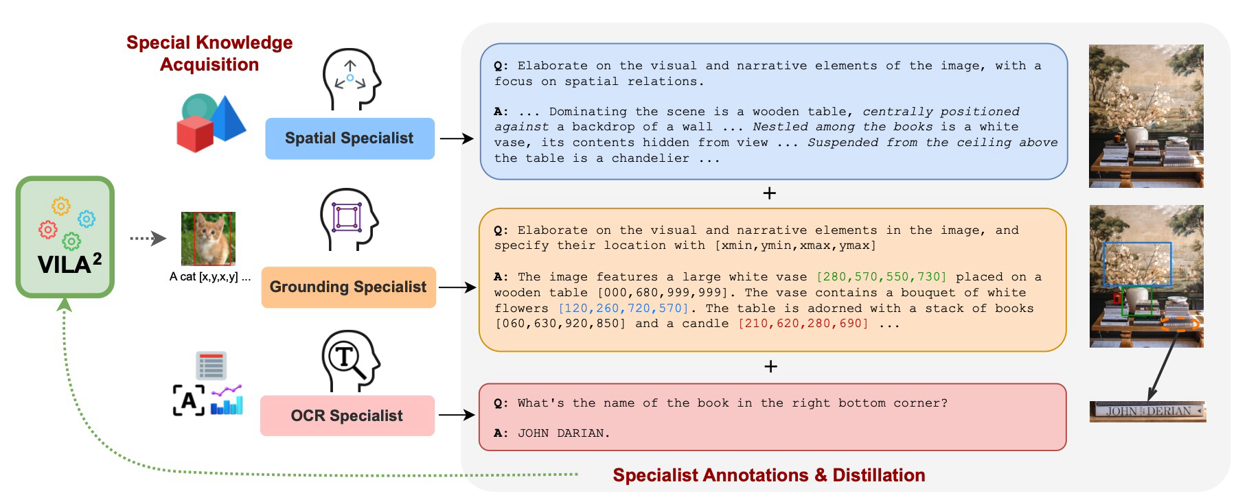
Table shows the ablation result on the effect of different specialist augmentation methods. Overall, specialist augmentation helps improve the model performance on several benchmarks.
| Method | VQAv2 | GQA | VQAT | POPE | SEED-I | MME | MM-Vet | MMMU |
|---|---|---|---|---|---|---|---|---|
| 10% MMC4-core + 10% COYO-25M + ShareGPT4V-Pretrain | ||||||||
| Original Caption | 81.4 | 63.8 | 65.2 | 85.5 | 70.6 | 1472.5 | 34.0 | 31.8 |
| +Spatial Specialist | 81.9↑0.5 | 64.1↑0.3 | 66.0↑0.8 | 85.9↑0.4 | 71.8↑1.2 | 1476.5↑4.0 | 36.7↑2.7 | 32.5↑0.7 |
| +OCR Specialist | 81.8↑0.4 | 64.0↑0.2 | 65.3↑0.1 | 86.4↑0.9 | 72.1↑1.5 | 1500.2↑27.7 | 34.3↑0.3 | 32.1↑0.3 |
| +Grounding Specialist | 81.8↑0.4 | 64.0↑0.2 | 65.1↓0.1 | 86.7↑1.2 | 71.0↑0.4 | 1536.4↑63.9 | 37.5↑3.5 | 32.6↑0.8 |
| MMC4-core + COYO-25M + ShareGPT4V-Pretrain | ||||||||
| Original Caption | 82.2 | 63.9 | 66.7 | 86.5 | 71.2 | 1518.2 | 42.6 | 33.4 |
| +All 3 Specialists | 83.0↑0.8 | 64.7↑0.8 | 70.9↑4.2 | 86.4↓0.1 | 74.0↑2.8 | 1656.2↑142 | 44.7↑2.1 | 35.8↑2.4 |
VILA\(^2\) is trained using a common three-stage align-pretrain-SFT paradigm, including initializing the projector, pre-training vision-language using both interleaved image-text data and image-text pair data (with the rewritten captions). Finally, visual instruction tuning is applied. VILA\(^2\) is ranked among the most performant models among open-source VLMs. The figure below compares the performance of VILA\(^2\) across various benchmark. The authors also show that data quality matters more than computation. In particular, VILA\(^2\) for one additional epoch does not improve the performance, while increasing the data quality (by rewriting the caption using VILA itself) significantly boosts the performance compared to training with one more epoch.
LongVILA
LongVILA [13] addresses the challenge of processing long context in terms of the pipeline and the system. On the pipeline side, LongVILA introduces two new training paradigms including long context extension and long video-supervised fine-tuning. On the system side, they propose long-context Multi-modal Sequence parallelism (MM-SP) to parallelize video training and inference to further utilize the GPU computation.
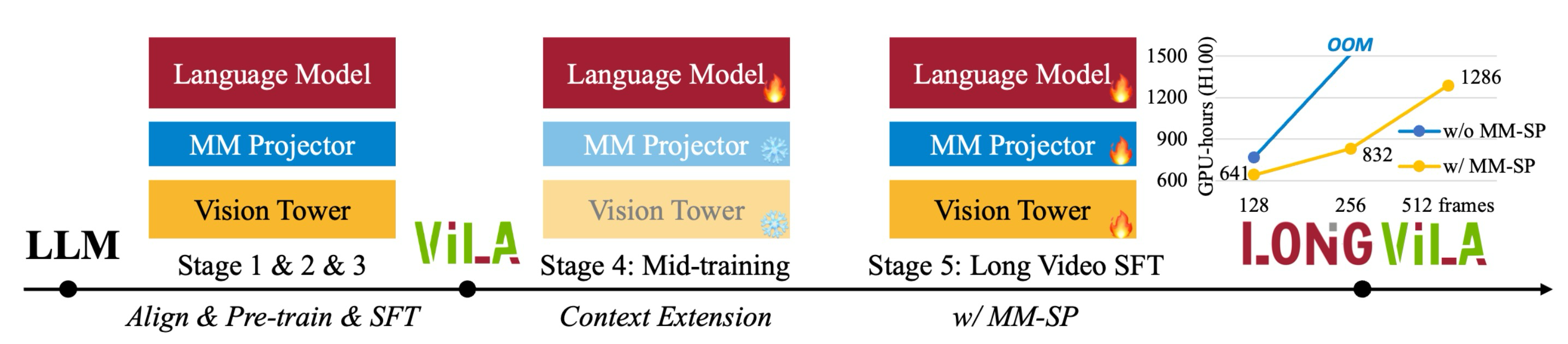
In LongVILA, there are five training stages; including 1) multimodal alignment; 2) large-scale pre-training; 3) short supervised fine-tuning; 4) context extension for LLMs; and 5) long supervised fine-tuning.
The first three stages are similar to that of the VILA model:
In stage 1, only the multimodal projector is trained.
In stage 2, the vision encoder is frozen and the LLM and multimodal projector is trained. VILA\(^2\) is applied to improve the dataset quality.
In stage 3, the model is fine-tuned with instruction-following data with images and short video datasets.
In stage 4, the LLM is pre-trained with text-only dataset to extend the context lengths. The LLM is progressively trained with different context length, ranging from 8192 to 262144.
In stage 5, the proposed MM-SP system is used to enhance the instruction-following ability, and all of the parameters are trainable in this stage.
Training data
LongVILA adopts the VILA\(^2\) method to first re-caption the images in the COYO dataset using the VILA model itself. In the supervised fine-tuning process, YouCook2 and ShareGPTVideo is used to train the model for short video comprehension.
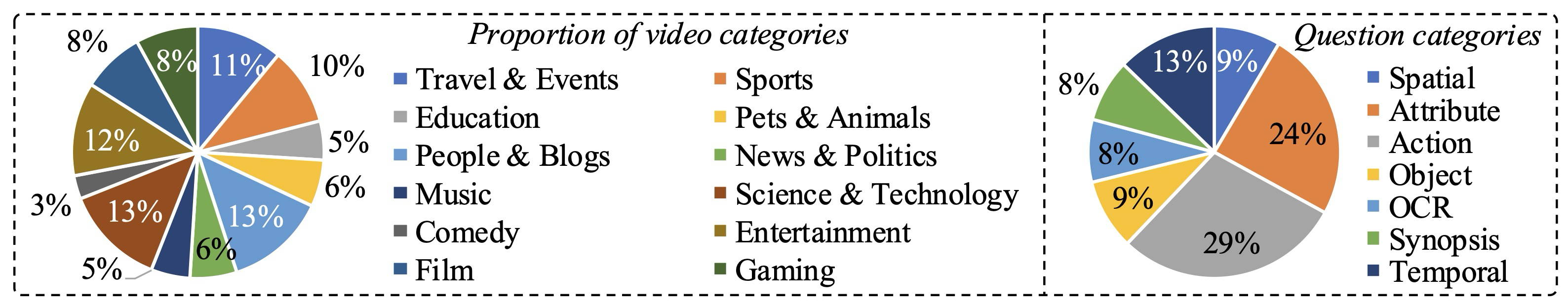
In addition, a new dataset consisting of over 15 thousands videos is introduced for long video instruction following in stage 5 of the model training process.
Multi-modal Sequence Parallelism
Previous methods of processing long context length have two limitations, one is modality heterogeneity and the other is networking heterogeneity. For Modality Heterogeneity, the text tokens are easy and fast to process, while visual tokens (like images or video frames) are more complex and require more resources. This can lead to an imbalance in GPU workloads, where some GPUs do much more work than others. For Networking Heterogeneity, GPUs that are close together (within the same machine) communicate very fast using NVLink, but GPUs that are far apart (across different machines) communicate more slowly using InfiniBand. This speed difference can create bottlenecks, slowing down the system.
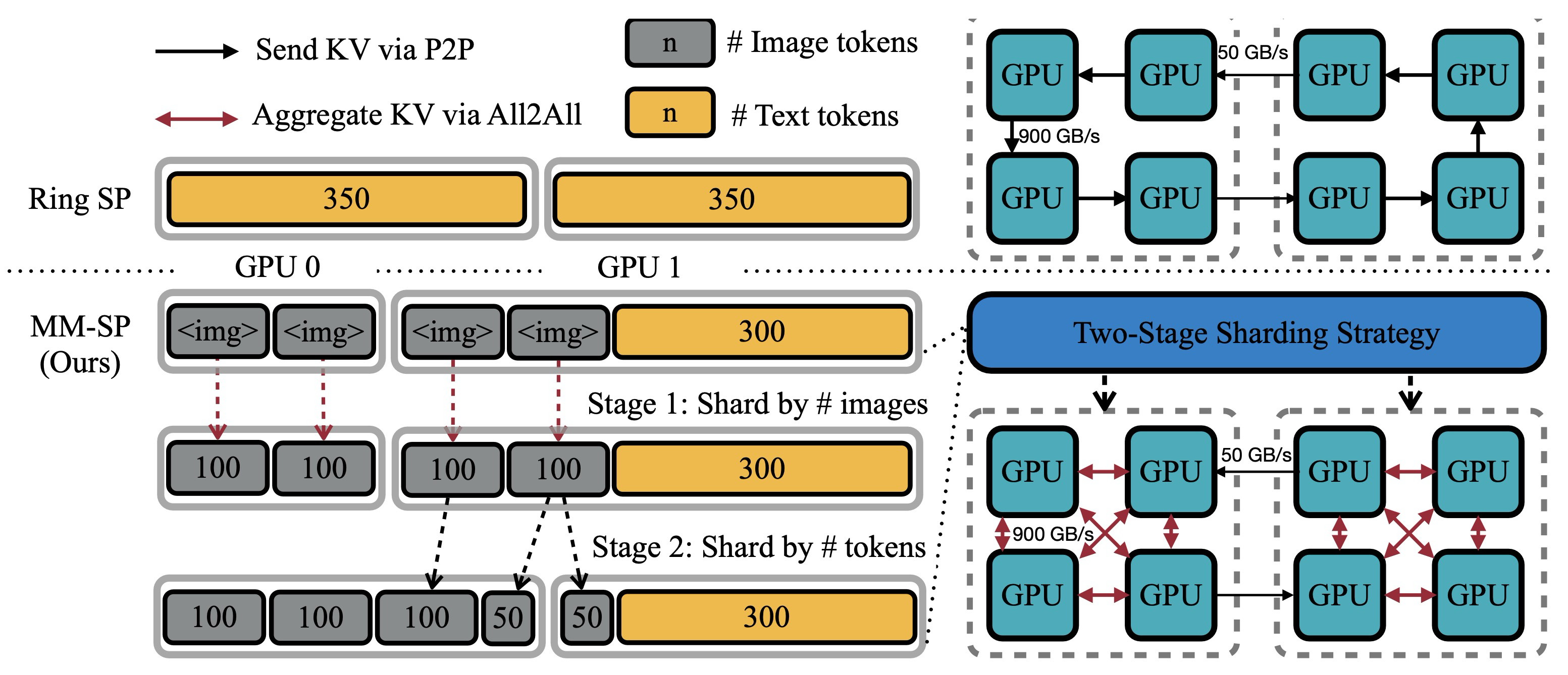
The two keys techniques adopted to address the aforementioned challenges are 2D-Attention [14] and two-stage sharding to distribute the work more evenly across multiple GPUs. The 2D-attention mechanism optimizes communication by organizing GPUs into a two dimensional mesh: intra-node communication is handled by splitting data along the attention head dimension, while inter-node communication transfers partitioned data chunks between GPUs. This structure ensures efficient and balanced computation.
To handle modality heterogeneity, the two-stage sharding strategy first distributes images evenly across GPUs for the image encoding stage. Then, in the second stage, it aggregates vision and text inputs, distributing tokens evenly for language modeling. This approach balances workloads across GPUs and maintains consistency using techniques like dummy token padding. For inference, the authors implement a system where all GPUs operate concurrently, avoiding bottlenecks in traditional methods like HuggingFace Pipeline Parallelism. This allows for efficient use of memory and computation, enabling the handling of longer sequences and faster processing.
VILA-U: A Unified VLM
At its core, VILA-U [15] is built upon two main principles: 1) creating an end-to-end autoregressive VLM that is able to generate images along with textual input alignment (instead of just trying to reconstruct the images); and 2) autoregressive image generators can create images that is of comparable quality to diffusion models as long as it is trained on a high-quality image-text dataset.
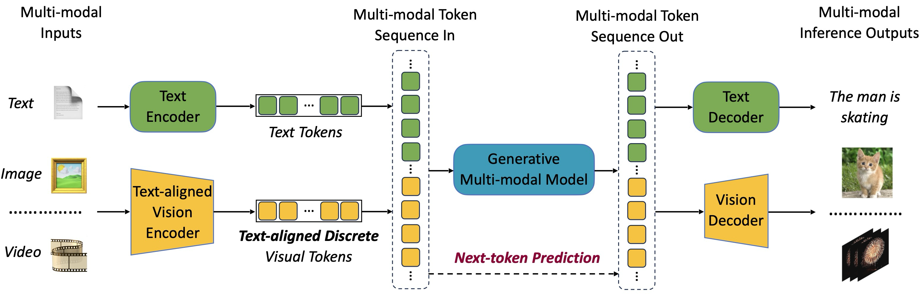
While developing a generative VLM is not new, previous works often offload the generation task to a seperate model, either Diffusion model [16, 17] or combining VQ-GAN and LLM [18]. The key novelty in VILA-U is its unified approach to visual and text generation. It adopts a next-token prediction method for both text and visual content generation. Visual inputs are tokenized into discrete tokens and concatenated with textual tokens into a multi-modal token sequence. The visual input tokens are discretized using residual quantization. Both text and visual input tokens are, therefore, discrete, and thus we can train the LLM with next-token prediction task. The authors use special tokens: <image_start> and <image_end> for images; <video_start> and <video_end> for videos, with video tokens formed by concatenating image tokens.
This unified token sequence is then processed during training with a single next-token prediction objective, allowing the model to learn both text and visual generation in an integrated fashion.
Residual Vector Quantization
The visual inputs are first tokenized into discrete tokens, as shown in the figure below. These tokens are then concatenated with the textual tokens, forming a multimodal token sequence. Then, all of these tokens are used to train for next-token prediction task.
To efficiently discretize the visual input tokens, the authors adopt a Residual Vector Quantization (RVQ) method as proposed in RQ-VAE. Given an input vector \(\bf{z}\), we want to represent it as a sequence of \(D\) discrete codes:
\[ RQ(z; C, D) = (k_1, \cdots, k_D) \in [K]^D \]
where \(C\) is a codebook that contains a set of \(K\) pre-defined vectors (also referred to as code), \(D\) is the number of quantization step, and \(k_d\) is the code selected from the codebook at step \(d\). Then, the RVQ breaks the vector \(\bf{z}\) into residuals across \(D\) steps, where at each step \(d\), it would first compute the code \(k_d\) by finding the closest match to it from the codebook:
\[ k_d = Q(r_{d-1}, C) = \underset{k \in [K]}{\text{argmin}} \|r_{d-1} - e(k)\|^2, \]
where \(e(k)\) is the embedding of the code \(k\), and \(r_{d-1}\) is the current residual. Then, we would update the residual as follows:
\[ r_d = r_{d-1} - e(k_d) \]
This step is repeated for \(d=1,2, \cdots, D\) steps, starting with \(r_0=z\). Finally, the approximated vector \(\hat{\bf{z}}\) of \(\bf{z}\) is computed as:
\[ \mathbf{\hat{z}} = \sum_{i=1}^D e(k_i) \]
Generative Pre-training
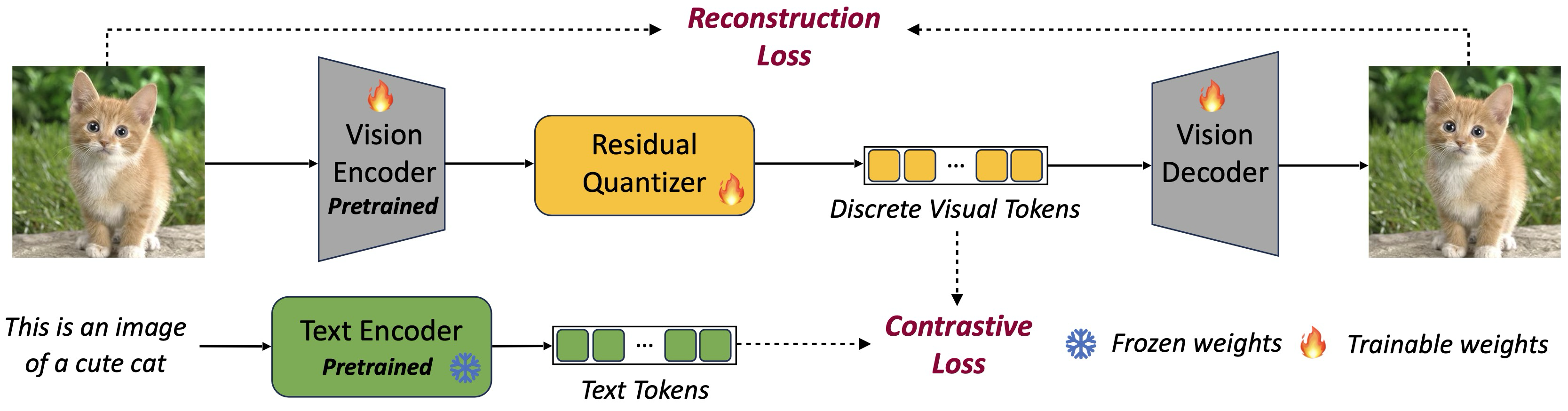
To achieve text and discrete visual token alignment, the authors propose using text-image contrastive loss along with VQ-based image reconstruction loss to equip the model with image generation capabilities.
However, while text-image contrastive loss requires the high-level understanding, reconstruction loss require low-level features. Therefore, naively training the vision tower from scratch to optimize those two objectives simultaneously would lead to conflicting goals. In fact, training a vision tower that way would lead to only 5% accuracy on zero-shot ImageNet classification. The training approach for the vision tower is, therefore, to first initialize it with CLIP weights for text-image alignment, and then freeze the text encoder to train only the visual encoder with both contrastive and reconstruction loss:
\[ \mathcal{L}_{\text{total}} = w_{\text{contra}} \mathcal{L}_{\text{contra}} + w_{\text{recon}} \mathcal{L}_{\text{recon}} \]
Various training approaches have been attempted, but each faces significant challenges. Loading pre-trained CLIP weights into the text encoder and RQ-VAE weights into the vision encoder and decoder while training the rest of the model from scratch fails due to the absence of pre-trained CLIP weights for the vision encoder. Another approach is to freeze the vision encoder prevents learning crucial low-level features needed for reconstruction. making the text encoder trainable leads to instability in the early stages as chaotic quantized features and contrastive loss disrupt its weights, slowing down training overall.
Since both visual tokens and text tokens are discrete, we can train our LLM with the general language modeling next-token prediction objective. However, due to the use of residual quantization for visual tokens, the training objectives for text and visual tokens differ slightly. For text tokens, the negative log-likelihood loss is calculated as:
\[ \mathcal{L}_{\text{text}} = -\sum_{i=1}^T \log P_\theta(y_i \mid y_{\lt i}), \]
where \(T\) is the length of the multi-modal sequence, and \(i\) only counts when the text token appears at position.
For visual tokens, residual quantization introduces a depth-stacked structure of codes at each visual position \(j\). Specifically, given the code embedding \(h_j\) generated by the LLM for visual tokens at position \(j\), the depth transformer autoregressively predicts \(D\) residual tokens \((k_{j1}, \cdots, k_{jD})\). During training, the input of the depth transformer \(v_{jd}\) at depth \(d\) is defined as the sum of the code embeddings of up to depth \(d-1\) for \(d>1\), such that \(v_{jd} = \sum_{d'=1}^{d-1} e(k_{jd'})\) and \(v_{j1} = h_j\). Thus, the depth transformer predicts the next code for a finer estimation of the feature \(\hat{z}_j\) based on the previous estimations up to \(d-1\). The negative log-likelihood loss for visual tokens is: \[ \mathcal{L}_{\text{visual}} = -\sum_{j=1}^T \sum_{d=1}^D \log P_\delta(k_{jd} \mid k_{j,\lt d}), \]
where \(T\) is the length of the multi-modal sequence, and \(j\) only counts when a visual token appears at position \(j\). During the multi-modal pre-training, the weights of the depth transformer are randomly initialized and updated together with the LLM.
| Model | Pretrained Weights | Resolution | Shape of Code | rFID↓ | Top-1 Accuracy↑ |
|---|---|---|---|---|---|
| VQ-GAN | – | 256 × 256 | 16 × 16 | 4.98 | – |
| RQ-VAE | – | 256 × 256 | 8 × 8 × 4 | 3.20 | – |
| RQ-VAE | – | 256 × 256 | 16 × 16 × 4 | 1.30 | – |
| VILA-U | SigLIP-Large | 256 × 256 | 16 × 16 × 4 | 1.80 | 73.3 |
| VILA-U | SigLIP-SO400M | 384 × 384 | 27 × 27 × 16 | 1.25 | 78.0 |
NVILA
NVILA [19] is a model built on top of VILA to improve the training efficiency regarding both algorithm and system side while maintaining the model’s performance. In the paper, the authors propose using data pruning and FP8 mixed precision training method.
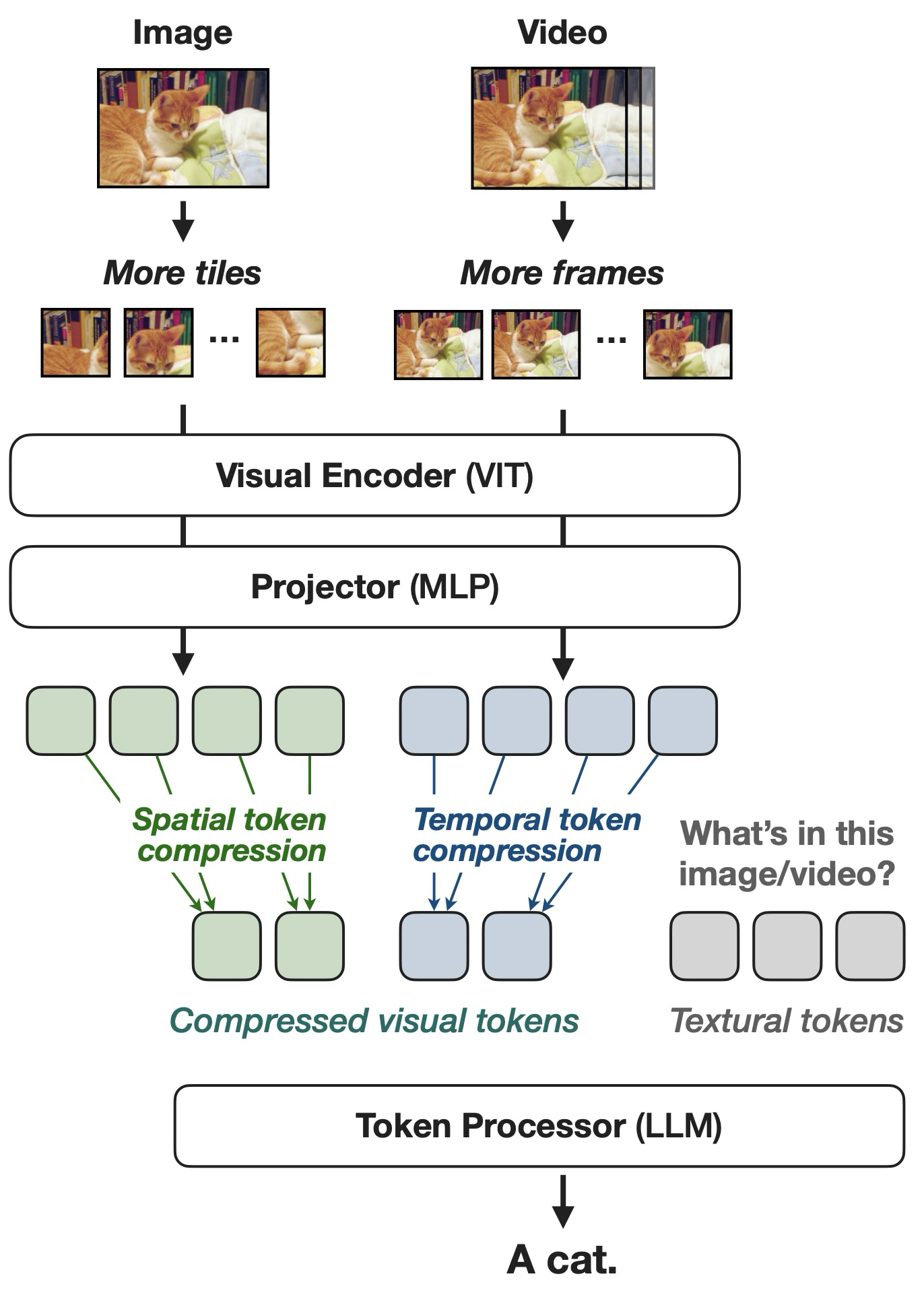
Scale-and-compress scheme
The scaling is to preserve the visual features, while compress is to reduce the computation. The compressed visual tokens are expected to be information dense, as visual tokens are often found to be redundant [20, 21]. In this paper, the two types of visual token scaling are spatial and temporal, whe`re spatial means to increase the image resolution and temporal means to increase the number of frames sampled from the video.
Visual token compression
One way to compress the visual token is \(S^2\) [22]. Each image is first resized to be of different resolution: 448x448, 896x896, 1344x1344. Then, each image is splited into different tiles that have resolution of 448x448. The feature map of the tiles from the vision backbone will then be concatenated. However, resizing all of the image to be square might lead to distortion.
| Model | Spatial Pooling | #Tokens/Tile | #Tiles/Image | AI2D | DocVQA | TextVQA | Image-10 |
|---|---|---|---|---|---|---|---|
| Baseline (VILA-1.5) | 2×2 | 256 (16×16) | 1 | 87.0 | 61.3 | 67.5 | 61.2 |
| Scale (Dynamic-S2) | 2×2 | 256 (16×16) | 9-12 | 90.1 | 91.1 | 77.0 | 71.5 |
| Scale + Compress | 3×3 | 121 (11×11) | 1-12 | 87.4 | 82.3 | 74.1 | 67.1 |
| Scale + Compress + VEP | 3×3 | 121 (11×11) | 1-12 | 89.8 | 88.8 | 76.1 | 70.8 |
| Alternative Designs | |||||||
| TokenLearner | – | 121 | 1-12 | 90.0 | 86.5 | 75.6 | 69.8 |
| Perceiver Resampler | – | 121 | 1-12 | 76.8 | 71.8 | 65.3 | 59.4 |
Therefore, Dynamic-\(S^2\) is proposed to resize the image to the resolution that is closest to the original solution that is divisible by 448. Using Dynamic-\(S^2\), the model performance can improve up to 30% on text-heavy tasks, as shown in Table 10.
Efficient training
The NVILA training process consists of five stages: projector initialization, visual encoder pre-training, token processor pre-training, image instruction-tuning, and video instruction-tuning. Stages 1, 3, and 4 are similar to VILA, while stage 2 focuses on maintaining model accuracy after visual token compression, and stage 5 improves the ability to process long videos. Similar to LongVILA, NVILA aims to improve the training efficiency both on the algorithm and the system side with data pruning using Deltaloss [23] and FP8 mixed precision technique. Given that the dataset used to train NVIA involved over 100M samples, data pruning is essential. In NVILA, Deltaloss is used to prune the data in an unsupervised way. The Deltaloss is defined as:
\[ D' = \bigcup_{i=1}^k \text{top-K} \left\{ \log \dfrac{p_{\text{large}}(x)}{p_{\text{small}}(x)} \big \vert x \in D_i\ \right\} \]
Here, \(D_i\) is the i-th subset of the fine-tuning dataset and \(D'\) is the pruned training dataset. According to the ablation study, 50% is a safe threshold in a way that it does not hurt accuracy so much while speeding up the training time to \(2 \times\).
FP8 training
FP8 precision offers significant benefits in computational and memory efficiency, supported by new NVIDIA GPUs like the H100 and B200. It accelerates training by performing matrix multiplications in FP8 and quantizing gradients, weights, and momentum, reducing memory usage and communication overhead.
| GC | BS | Throughput | MMMU | Video-MME |
|---|---|---|---|---|
| ✗ | 4 | 199.2 (1.0×) | 47.9 | 52.9 |
| ✗ | 16 | 390.1 (2.0×) | 47.0 | 53.0 |
| ✓ | 30 | 491.7 (2.5×) | 47.8 | 53.1 |
| ✓ | 36 | 579.9 (2.9×) | 47.7 | 53.0 |
For NVILA, FP8 allows increasing batch size, resulting in a 2x speedup. In VLM training, where sequence lengths vary widely (e.g., video tokens vs. image tokens), FP8 helps optimize performance. When gradient checkpointing is used, FP8 still provides a 1.2x speedup over BF16 training. Overall, NVILA is found to rivals with top-tier proprietary models like GPT-4o or Gemini 1.5. Pro, and sometime even surpasses them.
Acknowledgments
Thank you TMA Solutions for providing the necessary compute resources for VILA1.5-3B model inference.